The IRS reads data in ramps with 4, 8, or 16 reads, which are used to calculate the slope image in electrons/s (among other uses, including cosmic ray rejection, linearity correction, etc.). Here we examine several different methods by which those reads can be used to estimate a slope, in the context of a Monte Carlo model which approximates the noise properties of real IRS ramps. The noise model includes only two components: the Poisson noise of the accumulating photo-electrons, and the read noise per sample. Note that the nature of the accumulating Poisson noise ensures that each read is correlated, in a random-walk type process, to all prior reads on the ramp (a property of time-series data points like stock prices which the statisticians call "serial correllation").
Given the number of samples in the ramp, the slope in e/s, and the read noise in electrons, the model creates sequentially a large number of sample ramps with the same input slope, by accumulating photo-electrons according to a Poisson distribution, and imposing a Gaussian read-noise on each read afterwards. Each ramp is then used to estimate the slope in four ways:
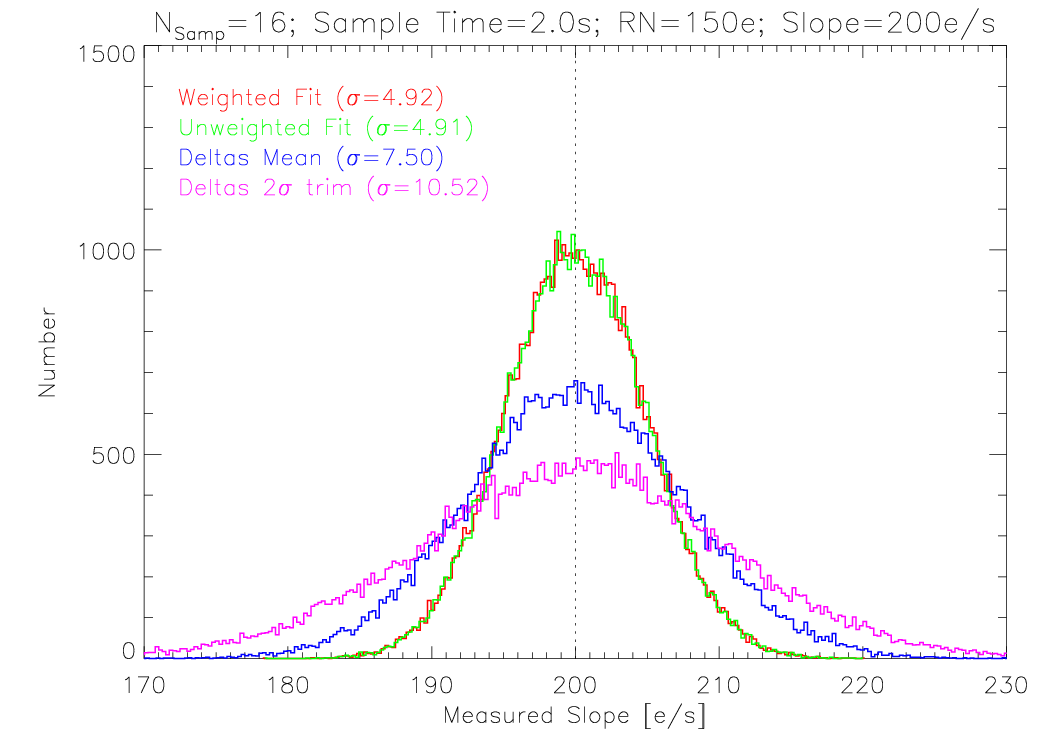
The distribution of recovered slope values yields information on the fidelity of the particular slope estimator. Here are the results for a particular exposure time of LL, 30s, with 16 reads, as a function of source brightness (slope). The read noise per sample was taken to be 150e. Each image shows the distribution of measured slopes for each of the 4 methods.
All four methods provide an unbiased estimate of the slope, in that they peak at the known input value. The width of the distribution varies considerably. At this low slope level of 200e/s (roughly the zodiacal value, which sets the lower threshold), the linear fit is ~50% better at recovering the input slope than the mean, with a width of 4.9e/s vs. 7.5e/s. It is over 2x better than the sigma-trimmed mean.
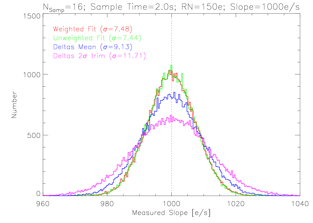
As the source flux increases (here to the level of a multi-Jy source), the mean becomes a less noisy estimator, but is still somewhat inferior to the linear fit.
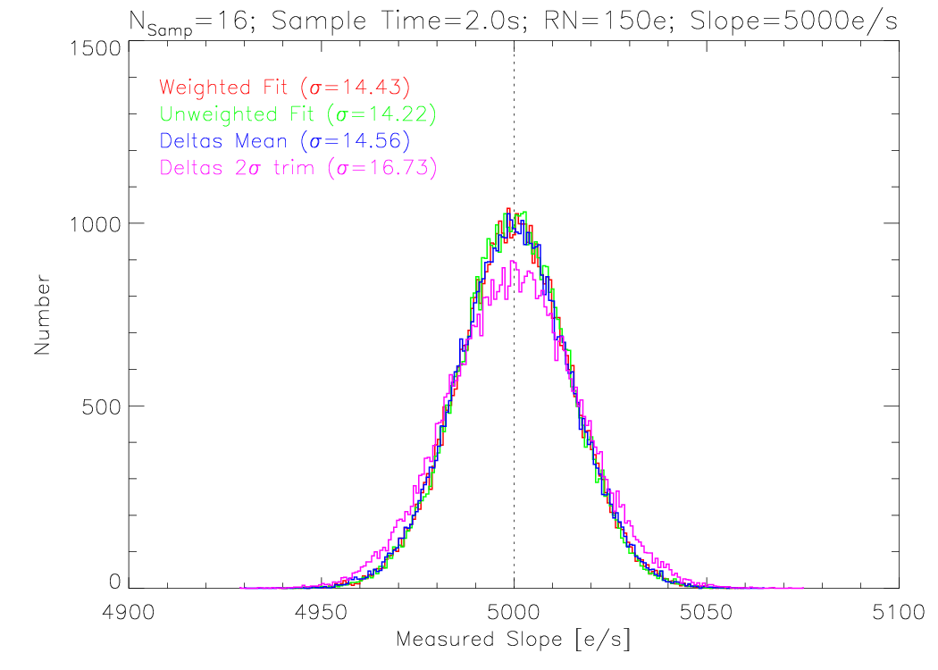
At the very high source flux of 5000e/s, which saturates near the end of ramp, the mean and linear fit are nearly identical. The relative error for all methods is quite small; the differences between these methods is most apparent at low source flux. Also available are model runs for other exposure time combinations:
The counter-intuitive result that sigma trimming actually worsens the estimate holds true because all points were drawn from a pure gaussian distribution of read noise. Trimming is effective at improving an estimator when it is expected that some measured points deviate wildly, far more than the Guassian probability would permit. This model does not address that concern, but the strongest source of deviation, cosmic rays, are treated before the slope is estimated. Even then, the mean of all points (0 deviates rejected) is a less precise estimator of the slope than the linear fit. At the very brightest end of the longest ramps, the mean can actually perform better than the line fits, since it ignores all of the lower fidelity early samples. This case is not encountered in real IRS data.
Given a determination of the slope using the ramp data, estimating the error in that slope in the context of a linear fit cannot make use of the standard parameter errors of linear least squares fitting theory, since these rely on the independence of each sample measurement. Since the ramp samples are serially correlated, the calculation of the error in the slope must be modified; see Gordon et al., 2005 Appendix A for more information. An important point is that only the error in the slope is affected by the correllation. The slope itself is unchanged. In fact, the precision with which the slope is determined is independent of whether measurement weights are used in the least squares fit; accurately estimating the uncertainty in the fit does require applying predicted measurement errors.